How to create high quality orienteering base maps
Updated December 2019 to reflect changes to the Australian coordinate system.
Updated December 2023 with information about The Spatial Collaboration Portal and Topographic Maps access.
Updated March 2025 with information and links to STD Explorer which replaces Spatial Services SIX Maps.
CONTENTS
Preface
Introduction
Part 1 - Gathering the data
Compiled by: Barry Hanlon with contributions from Ian Miller and Janet Morris.
Software is upgraded often. Always check that you have the latest version.
The coordinate system for Australian maps has changed from GDA/MGA94 to GDA/MGA2020. For new maps and updates to existing maps it is recommended to use the new system, which takes into account continental drift. the difference between the old and new systems in NSW as at the beginning of 2020 is about 1.5 metres. The new system is more accurately aligned with GPS devices that may be used by mapping field workers. The information about setting up the coordinate system in QGIS and OCAD (Part 2, Step 2) has been updated to reflect the changes.
Resource Target: mapping novices.
Preface
This document is a guide and reference manual for those creating and updating orienteering maps. Barry Hanlon has extensive (unparalleled) experience in creating new maps and is congratulated for documenting his knowledge to assist future WHO map makers.
Mapping is a pleasurable pastime and skilled mappers are in great demand. Congratulations on getting this far and commencing your journey in mapping.
Ian Miller, WHO President
Important Information
There are a raft of terms and names that will be new to novice mappers. Please do not be daunted by them. You will soon sort out those that are interesting or important to you. The rest may be important another time.
OCAD Software and naming conventions
OCAD is a software program developed for drawing orienteering maps that has now extended into a commercially successful product used for a number of applications such as plotting council drains and power lines. OCAD is available as an on-line subscription application. WHO has a team licence for the current version of OCAD.
The OCAD program works by taking in images of the area from various sources to be used as “background maps” or directly, E.g. Shape files. "Background maps" are usually aerial photographs of the area being mapped, but they can be copies of old maps, school ground plans and other OCAD files, e.g. created from Open Street Map.
To create an Orienteering map, you use OCAD to trace the features on the background map. OCAD translates them into orienteering symbols.
The OCAD software has been the standard for the last 20 years. Recently a free open software product has become available. This is known as “Open Orienteering Mapper” OOM. OOM has similar drawing functions to OCAD but at the time of writing it did not have several of the functions needed for facilitating the production of base maps from spatial data such as Lidar.
Technology Advances
Over the last few years a number of technology advances help map makers create more accurate maps. For example: Geo-referencing points on the map places them correctly in relation to their location on the earth’s surface. Contour lines and rock features can now be mapped more accurately.
Mapping Process
The process usually involves two main steps – the creation of a “base” map using the available spatial resources (images and vector data) for the selected area followed by field-working. Field-working involves visiting the area and editing the features on the base map to match the real world. New features may have been added since the spatial resources were gathered (occurs frequently on urban maps) or the features may have changed (e.g. bush fire or clearance in a bush area).
Introduction
It makes the field worker’s job a lot easier if the base map they are given to work from has been prepared with the use of all available resources. These notes are intended to help mapping novices to access and use the extensive free spatial data resources that are available to create high quality base maps.
Firstly, we need to identify the available resources, how to access and use them to download spatial data. Our focus is on mapping beginners so we will look at the freely available resources. Mention is also made of NearMap – a commercial resource that can be accessed through ONSW’s Mapping Officer.
[Anything beyond these resources is really in the professional mapper domain and can be very expensive. E.g. if no Lidar is available a commercial flight would cost several thousand dollars (the development of drones may bring these costs down in the future).]
Secondly, we look at the ways these resources can be used to create base maps in OCAD (the latest version of OCAD has advanced Lidar processing which is continually being upgraded).
Finally, we look briefly at other mapping options such as Open Orienteering Mapper (free) and alternative ways of processing the data for use in OOM.
Part 1 – Gathering the data
You may have done some field work previously and are now starting a new map. Don't be daunted by the new names and tools you will learn about below, but please keep reading to the end before you come back here to start your mapping project!
Ask questions. The quickest way to learn is using the experience of others.
Project Folder
First create a project folder for your new map eg.: MyNewBaseMap. It is a good idea to create a set of sub-folders for the free spatial data you are going to download. A separate folder for each data source is a good idea.
Suggested sub-folders (under MyNewBaseMap):
For collecting the spatial data downloads
ELVIS (Lidar cloud .las files);
Google Earth (for downloaded aerial photos);
STD Explorer (also for downloaded aerial photos);
Clip and Ship (for the .shp files that you will download from Spatial Services);
Pullautin (for the .png format map graphics that Karttapullautin generates from .las files);
QGIS (for exported geo-referenced aerial photos from NSW Spatial Collaboration Portal (previously NSW Globe);
TopoMap (for graphic files copied from the topographic map of the area being worked on).
When you start to create the base map in OCAD you will need two more folders:
DEM (Digital Elevation Model - for the DSM, DTM DEM files that OCAD produces from the Lidar .las files and the geo-referenced graphics of the area that OCAD also outputs as background maps);
Logos (for any logos that need to be placed on the finished OCAD map).
The Free Resources
- STD Explorer - an online mapping and spatial information tool provided by NSW Spatial Services. [It replaced SIX (Spatial Information Exchange) in 2025.]
- NSW Spatial Collaboration Portal (replaced NSW Globe April 2020). The NSW Spatial Services spatial data base.
- Web Services. Access to georeferenced NSW Imagery provided by Spatial Services. Web services can be accessed by mapping software such as QGIS.
- QGIS. German software that can link to Web Services imagery database to produce geo-referenced aerial photographs.
- ELVIS. Lidar cloud resource.
- Open Street Map. Maintained by volunteers. A source of additional spatial information that is often useful.
- Topographic GeoPDF maps. High quality pdf versions of NSW Spatial Services topographic maps can be downloaded from NSW Spatial Collaboration Portal.
- SIX Clip & Ship. Cadastral and Topographic data in vector format. (Daya access may be replaced in the future by a subset of NSW Spatial Collaboration Portal)
- NSW Bushwalking Maps. Worth checking out but usually not very useful.
- Karttapullautin. Finnish command line software used to process Lidar clouds. A useful alternative to OCAD's lidar processing when Open Orienteering Mapper is the preferred mapping software.
- Near Map. Usually has more recent geo-referenced aerial photos than Spatial Collaboraton Portal. This is not a free resource but ONSW has an arrangement with the company for limited downloads. Very useful if there are recent developments in the area of interest. For more information about this resource or to lodge a download request contact the ONSW Mapping Officer (mapping@onsw.asn.au).
STD Explorer
New South Wales’s Spatial Digital Twin (SDT), Explorer, is a free spatial visualisation product designed to provide quick and efficient tools for visualising, validating, and interacting with spatial data. Explorer bridges a gap by offering a mid-level, user-friendly interface with enough functionality to support the majority of common workflows, empowering professionals to explore spatial data, validate findings, and communicate insights effectively.
STD Explorer is a part of NSW Spatial Collaboration Portal where publicly available aerial photographs and cadastral data of NSW can be viewed . Its output is not geo-referenced (it is not possible to download aerial photos with a world file). However, it is useful at the map drawing stage to confirm/identify spatial details.
NSW Spatial Collaboration Portal
The NSW Spatial Collaboration Portal allows users to search and discover the 10 NSW Foundation Spatial Data Framework (FSDF) themes.
It is an access point for Spatial Services’ comprehensive package of land and property services, which include property information, surveying and mapping. Access is publicly available but to make full use the service you may need to create an account at Spatial Services website.
Web Services and QGIS
First step is to install the latest version of QGIS on your computer. Go to: https://www.qgis.org/en/site/forusers/download and select the version for your computer. There are Windows, MAC OS-X, Linux, BSD and Android versions of the software. Always use the latest version.
The next step is to link QGIS to Spatial Services Web Services and follow the instructions.
The link you will load into QGIS should look something like this: http://maps.six.nsw.gov.au/arcgis/services/public/
NSW_Imagery/MapServer/WMSServer?
request=GetCapabilities&service=WMS ]
IMPORTANT. At the bottom right hand corner of the QGIS screen you will see an EPSG number. For the east coast of Australia from 1st January 2020 it should be 7856. If not, you need to reset it. Click on the number. A screen opens where you can reset the "Project Coordinate Reference System". In the middle panel "Coordinate reference systems of the world" you need to scroll through until you find this entry under "Australia": "GDA2020 /MGA zone 56 - EPSG:7856". When you have the correct system selected for your region you will see a map of Australia below with a pink outline of the area covered. (If you are working on a map further to the west you will need to select the GDA2020 zone that applies to that region.)
NB If you plan to field work with a GPS device you may be better off setting your map coordinates to UTM / WGS 84 Zone 56 South EPSG:32756. This is the Universal Tansverse Mercator system used by GPS devices world wide. There is no significant difference between the coordinates of GDA2020 and UTM / WGS 84.
QGIS will opens a link to Spatial Services database at Bathurst. You will be able to zoom into your area of interest. QGIS lets you export a geo-referenced (.jpg image with world file) aerial photo of the screen or a selected area.
When you have the area of interest on your screen click on "Project" at the top left of the screen (menu line). Scroll down to "Import/Export" and select "Export to Image" from the pop-out menu. You are given the option of downloading the whole screen (Map Canvas Extent) or downloading a selected area (Draw on Canvas). For the latter you select your area by dragging a frame around around it (marqueing). Set the required resolution, click on "Save" and follow the on screen instructions.
NB:The default resolution (usually 120 dpi) can be increased by resetting to it a higher level but there is a resolution limit. If you set it too high you will get a solid green image. If this happens just resave the image with a reduced resolution. It is preferable to use the highest possible resolution.
[QGIS can also produce GeoTiff files but these are huge files and while technically better they do not offer any real advantage to orienteering mappers over the .jpg + world file that QGIS can export as described above.]
ELVIS
Lidar data sets of NSW can be accessed via ELVIS (Geoscience Australia - Elevation and Depth - Foundation Spatial Data). http://elevation.fsdf.org.au/
Several datasets are available. Point Clouds are the best as they can be used to generate both DSM and DTM DEMs. The DEM datasets in ELVIS are ground level only but useful if the Lidar cloud is not available. The 5 metre data sets can be used to select surface data for selected areas and will provide reasonably good contours but nothing much else. However, they are small files compared with the full Lidar Clouds which can be as dense as 250 MB.
The Lidar Clouds cover areas 2 x 2 kms (4 km2). The two data sets covering the area where we live are:
Sydney201304-LID1-C3-AHD_3146262_56_0002_0002.zip (160.2 MB)
Sydney201304-LID1-C3-AHD_3166262_56_0002_0002.zip (158.1 MB)
The number in the middle identifies the south-west corner of the Lidar tile. The first 3 numbers are the Eastings and the last 4 numbers are the Northings, both in kilometres, (i.e. in the first tile above we have 314E and 6262N). The spatial grid is MGA (Map Grid of Australia). Most of the NSW East Coast is in MGA zone 56 – MGA is also closely related to the GPS referencing system (WGS84 / UTM Zone 56S for coastal NSW) which is used by hand held tracking devices such as Garmin which are useful tools when you come to do the field work.
When you have made your selection and placed your order ELVIS will email you a download link.
The downloaded tiles will be in .zip files which need to be unzipped at two levels. For each tile you will end up with a .las file (the Lidar cloud) and an .html file (technical information and instruction on how the use of the data should be acknowledged).
NB.: The free Lidar clouds obtained through ELVIS may not have enough points per square metre for the interpretation software (OCAD and Karttapullautin, OL Lase, etc., to render complex rock detail adequately. If the fine detail is required then a costly fly over may need to be considered.
Open Street Map
You can export an area in OpenStreetMap as a .osm file which is geo-referenced.
To use the .osm as a background map in OCAD 2018 create a special OCAD Topographic map file and use that as a background map in your orienteering map project.
To do this you select NEW in OCAD, then choose Topographic, city or leisure map. Then select under “Load symbol set from” OpenStreetMap 10,000.ocd. This OCAD map can be one of the background maps for your new orienteering map.
Open Street Map is of limited use but can help in identifying the location of some features that are not seen or difficult to see on aerial photos. I have found it useful for locating powerlines/poles and the locations of items such as bus stops which may have shelter structures that can be used as check-point locations, etc.
SIX e-topo
[Printed maps have been phased out, access to pdf versions is still available,]
High quality pdf versions of NSW Spatial Services topographic maps can be downloaded for free from: https://maps.six.nsw.gov.au/etopo.html
These are high quality .pdf files almost the same as the NSW Spatial Services printed topographical maps. Selected areas can be copied and used a background maps. They are not geo-referenced but the mapping grid is on them, so that are easy to position in OCAD. One useful feature of these maps is the magnetic deviation from grid north. This is found in the top right hand corner under the "scale" information. This datum is critical for correctly orienting your map to magnetic north.
An alternative source for topo maps can be found here.
SIX Clip & Ship
This is a Spatial Services free resource for vector cadastral and topographic data: https://maps.six.nsw.gov.au/clipnship.html
The cadastral lot and street data is very useful. It can almost automate the drawing of streets in urban street and park maps.
The best type of downloads for importing into OCAD are the shape files (.shp).
Pick the area you want by choosing the MBR option and marquee (select) the area of interest. In the options choose the "Projection" MGA Zone (eastern/coastal NSW is zone 56) and choose to have the output delivered as shape files (Format delivery). Then check "Cadastral". The rest of the data request form is self-explanatory.
You can also request topographic data, The topo files are useful for generating contours when good Lidar is unavailable (The contours are really not very good. They are similar to those found on the LPI topographic maps - but better than nothing!).
Spatial Collaboration Portal is an alternative source for cadastral and topographic data. It will probably replace Clip and Ship in the future.
NSW Bushwalking Maps
http://maps.ozultimate.com - Based on Spatial Services topographic maps. Of limited use.
Karttapullautin
https://github.com/karttapullautin/karttapullautin
This is Finnish command line software used to process Lidar clouds. OCAD processes Lidar very well. One of the outputs from Karttapulautin is in the form of a .png map that is a simulated orienteering map. It is a useful indication of runnability (open areas and the various shades of green in particular).
Just drag and drop your .las file onto the Karttapullautin .exe file. A command line box/window opens and Karttapullautin starts processing the Lidar. It can take some time.
The output .png files are geo-referenced and can be imported directly in OCAD as background maps. If you have several Lidar tiles and your computer is multi-cored you can process the Lidar tyles in batch mode. Eg.: If your cpu has 6 cores Karttapullautin will process six tiles simultaneously, one in each core, a huge timesaver.
For MAC users Apple have some information about running Windows on a Mac at: https://support.apple.com/en-au/HT201468
Karttapullautin is a Windows command line program. On a MAC the command line app is called Terminal, don’t use this. In Windows the equivalent of Terminal is the Command Prompt. To run it enter WindowsKey+R then type CMD and press enter. NB.: On a MAC you need to check which key is the WindowsKey equivalent.
Now that you have gathered most of the data you need, we are ready to open OCAD and start compiling our base map.
 Part 2 – Creating a base map in OCAD
OCAD has several tutorials on its website. Here is one you may like:
https://www.youtube.com/watch?v=KWqPWRS5nu8
OCAD has Lidar processing options, so it is the software of choice for this exercise.
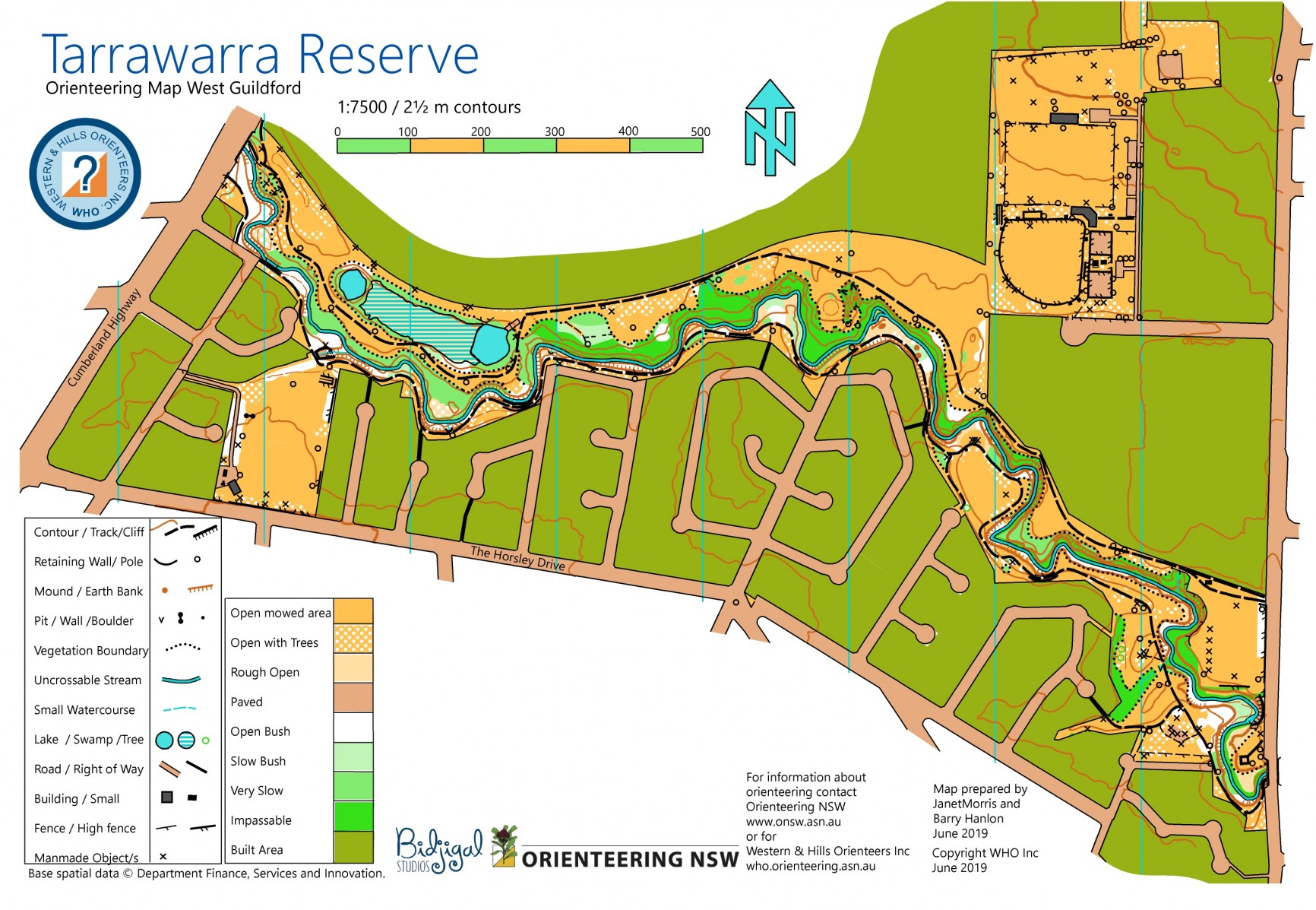
To demonstrate how we use OCAD to process our gathered resource data into a base map we need to select an area to map. Most of our new orienteering maps are of city streets and parks usually used for events such as the Sydney Summer Series. The demonstration area is a suburban area around Prospect Creek, centred on Tarrawarra Park. This has suburban streets, bike tracks, swamps, open and very green bush, sports fields, tennis courts, power lines, and much more.
Step 1 – Confirm the coordinates
The area we are interested in can be found on the Spatial Services “Prospect” topographic map, 9030-2N: (A digital version is available on Spatial Collaboration Portal.)
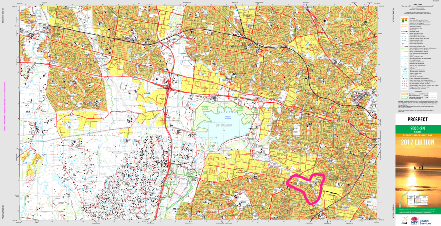
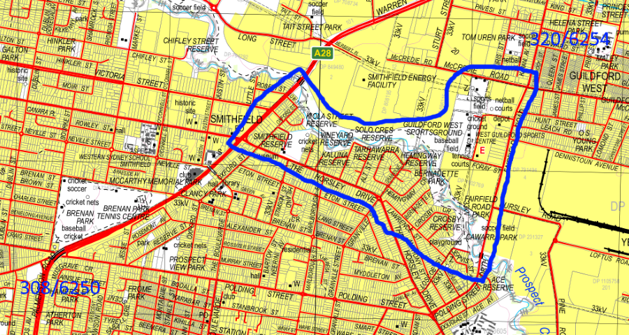
Zooming in we identify that the area is contained within MGA (Mapping Grid of Australia) UTM 56S coordinates 308/6250 and 320/6254.
These coordinates are selected because if Lidar is available the area of interest is covered by four tiles. The central coordinate is 310/6252.
Step 2 – Create a new OCAD Orienteering Map
The area fits neatly onto an A4 at 1:7500.
Open OCAD (You should always use the latest version) and create a new orienteering map using the most recent symbol set. Our map is going to be geo-referenced so we need to set the correct coordinates in OCAD.
Under OCAD's “Map” menu select “Set scale and coordinate system”. Select “Real-world coordinates” and enter the central coordinates in kilometres + 000 (= metres) plus the magnetic deviation (you can get this from the topo map) [for our example map the numbers are 310000 / 6252000 / 11.2]. At the bottom of the screen you will see the “Coordinate system” panel. Click on “Choose". In the next screen under "Coordinate system" select "Australia" then under "Zone"select "GDA2020 / MGA Zone 56". (MGA is short for Mapping Grid of Australia.) All Australian government mapping resources will be using this grid system from 1st January 2020. Using this coordinate system ensures that when we import Lidar, other geo-spatial information and field work tracks and way points from GPS devices (eg: Garmin hand helds) we are aligned. Zone 56 covers the east coast of NSW). {NB. Most GPS devices use an international system: UTM / WGS 84. We are in Zone 56 South. There is no significant diference between the international system and GDA2020 as far as orienteering maps go. You can use either coordinate system]
We have now set the coordinate system for our map. Click “OK”.
Under the “Map” menu select “Change scale”. Enter the new scale “7,500”. Select “Enlarge/reduce symbols”. This last bit is a matter of preference but selecting means that the symbols will in compliance with the IOF mapping standards. (NB: the IOF base scale standard for Orienteering maps is 1:15,000. The scale of 1:7,500 was chosen for this exercise to make better use of the area chosen for this project as it fits on A4. As a result, the symbol dimensions for our project will be double those set out in the standard. All mappers should be familiarise themselves with the standard, the latest version can be found on the IOF website.)
You now have a blank OCAD map.
The order of the actions set out in the next step is not critical.
Step 3 – Import the Clip & Ship data
[An alternative to Clip & Ship is through Spatial Collaboration Portal which allows you to be more selective with data types]
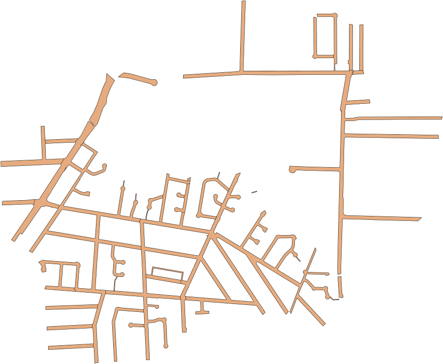
Under “File” / “Import” go to your “Clip and Ship” files. Select the “Road.shp” in the set of CAD files.
The cadastral data will be imported in unsymbolised form (red colour). Select any one of the imported shapes. In the “Select” menu choose “Select objects by symbol”, “All Objects in layer”, click “OK”. In the Symbol Box select the “Paved area symbol”. Click on the “Change symbol” icon on the tool bar.
You now have a map of the local streets, but it needs a bit of work to finish it. Make certain all the streets are selected. In the “Object” menu select “Merge”. The purpose of this is to reduce the graphic editing of the streets (every separate bit of a street will be bounded by a black line which needs to be edited out). Repeat the “Merge” a couple more times.
While all the streets are still selected, select the “Paved area boundary” symbol then click on “Fill or make border” on the tool bar.
You now have an almost automatically generated street map.
Other Clip and Ship data that could be useful can be seen in your downloads. They are processed in a similar way to streets. The topo download has contours. They can be useful but if Lidar is available OCAD will produce better ones. The hydrolines are usually inaccurate. Sometimes there will be electricity transmission lines which may give the location of towers. The cadastral “lot.shp” is also a useful file as it will contain the surveyed boundaries of parks and reserves.
If your only source of contour data is the contour shape file you process in much the same way. The following picture shows the raw unedited imports for contours, electricity power lines and hydro features.
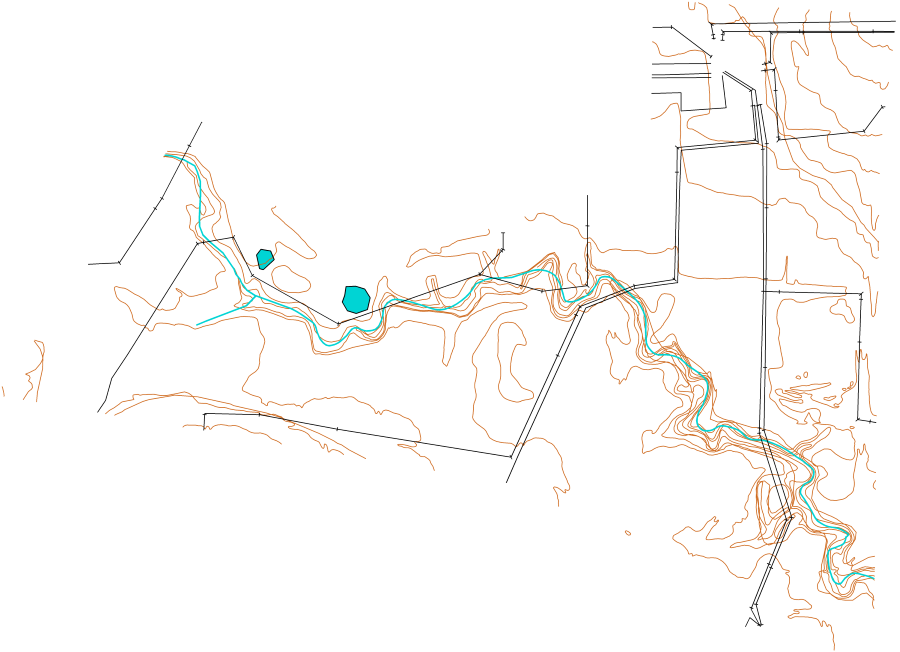
Lot boundaries can be imported – useful at the early stages of drawing the base map, but too detailed for the final version.
Step 4 – Processing the Lidar cloud in OCAD
Draw, with any line symbol, a rectangle, aligned to the MGA grid that includes the intended boundary of the finished o-map and select it.
Open the “DEM” menu and click on “DEM import wizard”. Under “Importable files – Add”, load the four .las files (the Lidar clouds). The selected rectangle will determine the limits of the objects created by the DEM import wizard (this reduces the size of the Lidar output). Click on “Next”. Under “File name:” click on the button and select the “DEM” folder you created earlier. Uncheck “Create Hypsometric Map” (not useful). Check “Create Vegetation base map” (can be useful for indication of runability and vegetation density). Click on “Next”. You probably won’t want to change any of the LAS Settings (DTM stands for Digital Terrain Model = ground level. DSM stands for Digital Surface Model = the upper level of the cloud). Click on “Next”. Under “Create Contour Lines” you probably want to select “Create smoothed contours” and deselect the other option. The default contour interval is 5 metres but you can reset this if another interval is more suitable for a particular map (I used 2.5 metres for this demonstration). Choose the contour symbols (use the standard ones).
OCAD will start analysing the Lidar. Contours will be created and depressions indicated. Several background maps will be created. All this can take a few minutes, but eventually you should see something like this:
:
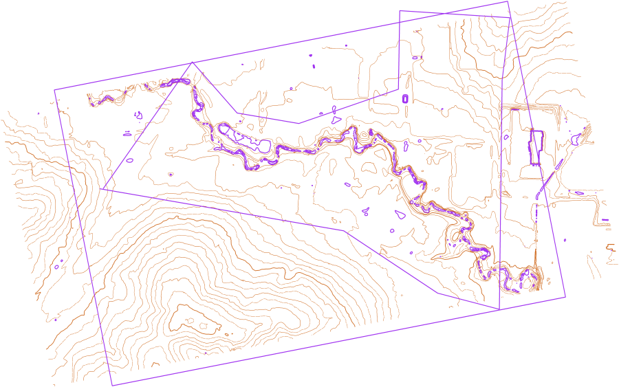
Press F10 to turn off the Lidar backgrounds. You will see the contours with depressions indicated by purple lines (I selected purple to highlight the depressions).
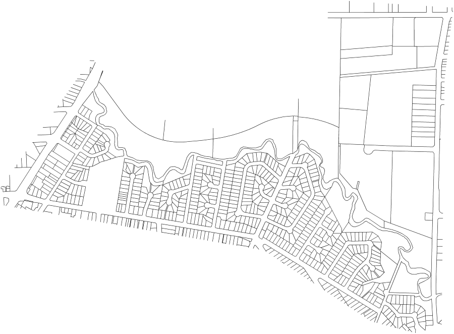
The above was then cropped back to the intended map area with streets, power lines, hydro features and cadastral boundaries we created from the shape files made visible:
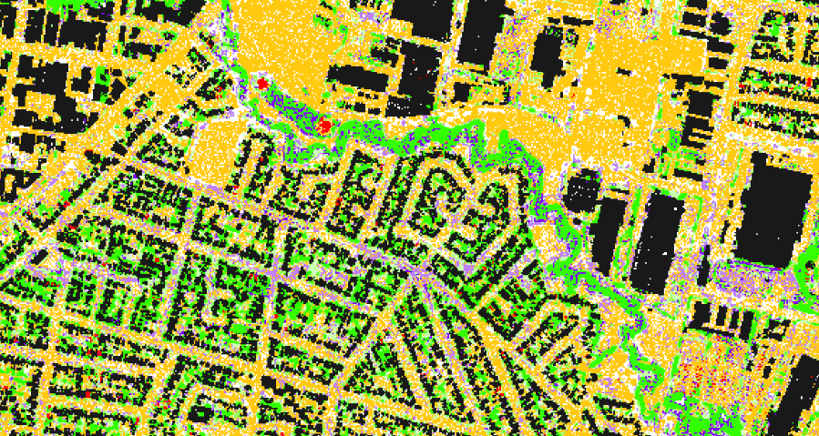
OCAD 2018’s Lidar processing produced these background maps:
Vegetation height classification:
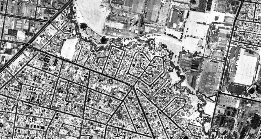
LAS intensity:
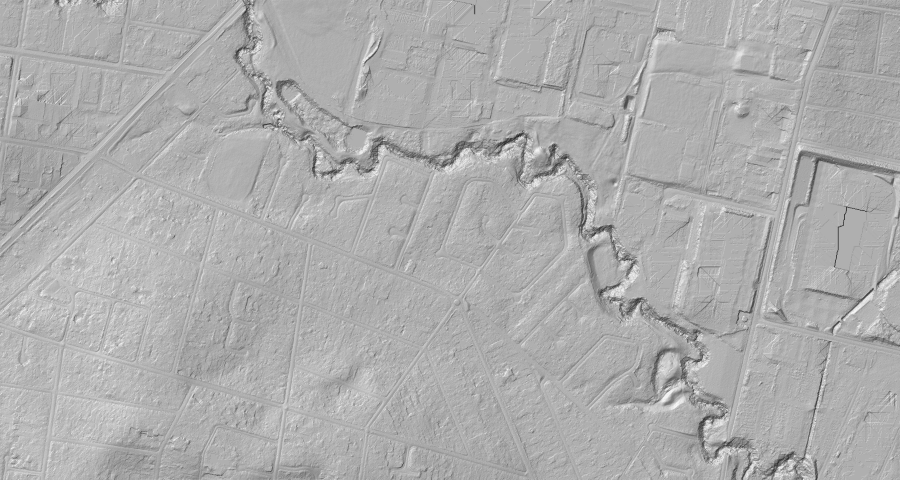
Hill shading:
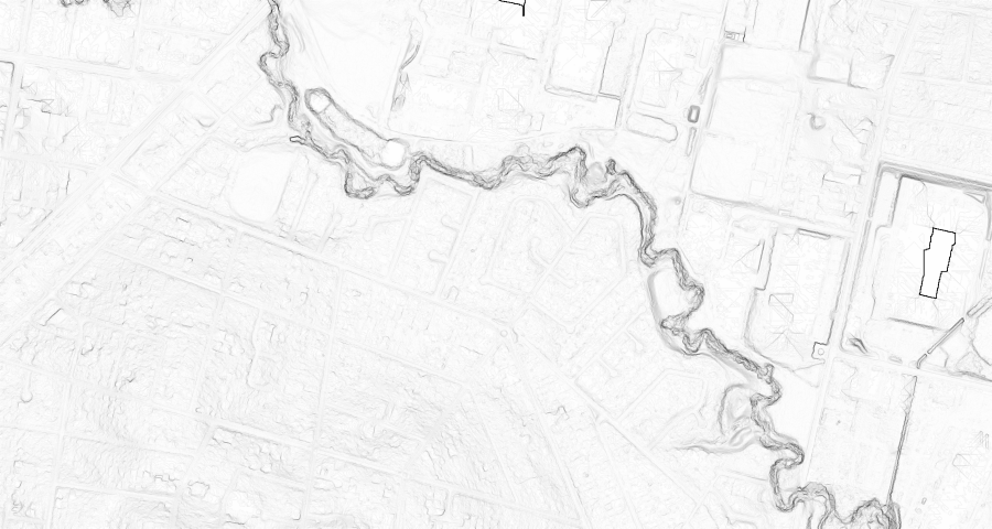
Terrain slope gradient:
LAS classification:
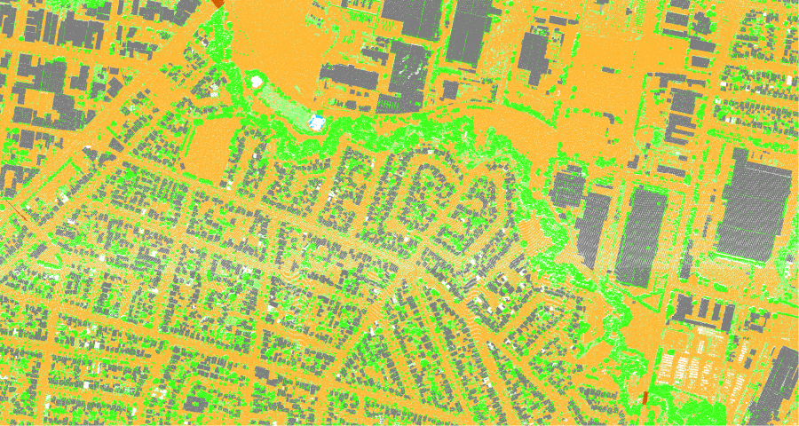
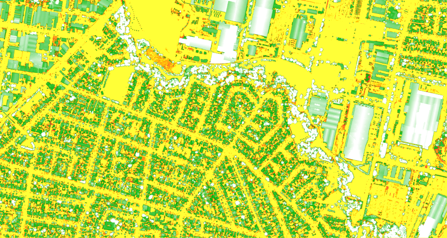
Simulated orienteering base map (two shades of purple indicates two levels of difficult running due to the probability of undergrowth) :
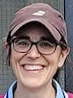
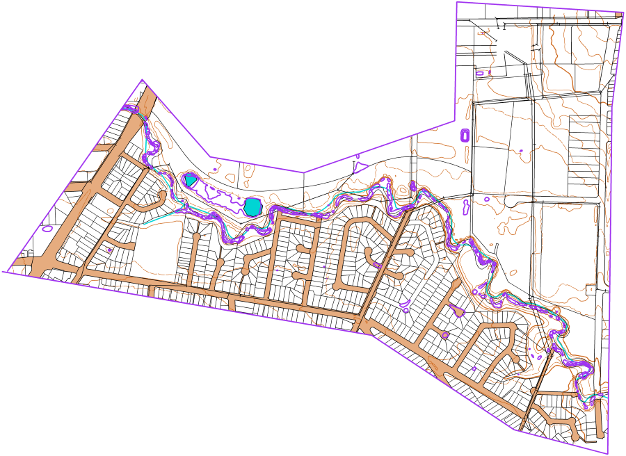
After a little bit more work in OCAD we end up with a base map for the field worker.
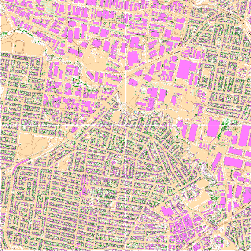
Karttapullautin
This is an extra step. It is not essential, but the Finnish software produces a simulated orienteering map that provides a useful check for runability. Its green shading and stripes are, in my opinion, clearer to interpret than OCAD’s output.
You can download the latest version of Karttapullautin from GitHib.
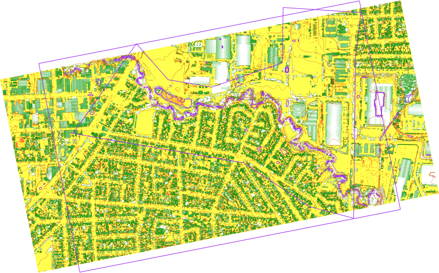
Pullautin process the Lidar tiles individually (there is a batch mode if you have a lot to process). The output is a montage of the four 2 km2 Lidar tiles that cover the area of interest, rendered by the Finnish software as .png files and assembled in the graphic below.
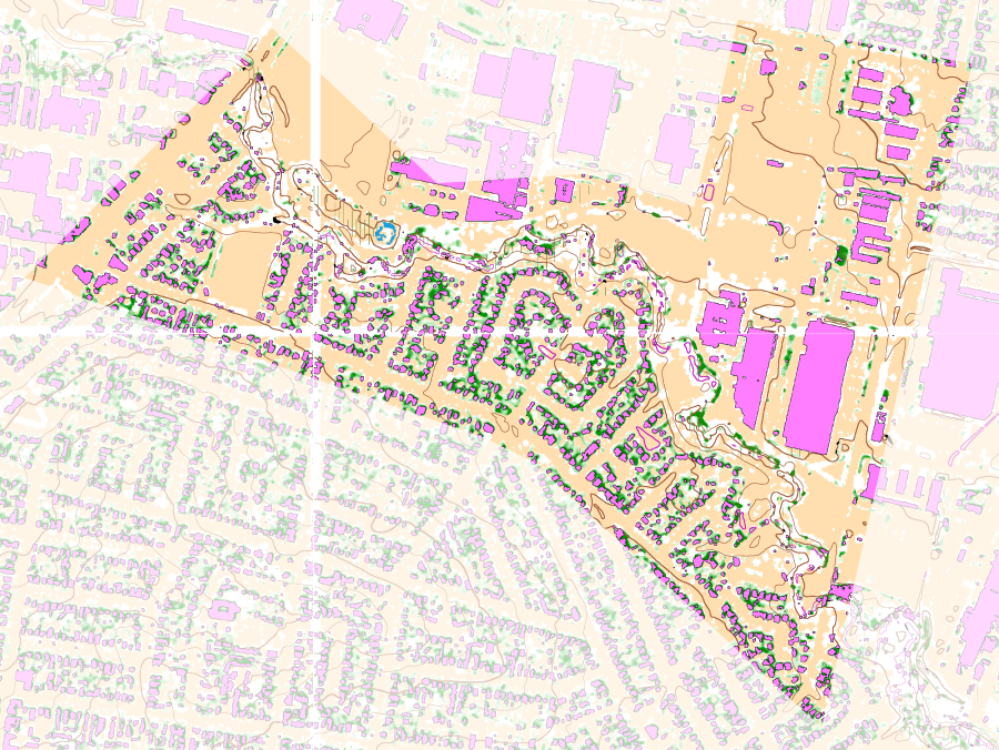
The area of interest is in the right hand centre of the picture:
To make the area of interest a bit clearer it is highlighted in the next graphic.
Part – 3 Alternative mapping tools
If you have access to the latest version of OCAD you won’t need to read this.
 Open Orienteering Mapper
https://www.openorienteering.org/
A good alternative to OCAD for drawing maps. It does not have Lidar processing tools but it processes .shp files as well as OCAD. The background maps produced by Karttapullautin can also be used as background maps in OOM. There would be a learning curve for anyone switching from OCAD but it would not be very steep.
There are tutorials on YouTube:
https://www.youtube.com/watch?v=n9ilQu1sBdo
https://www.youtube.com/watch?v=yA_GzECa-ZE
https://www.youtube.com/watch?v=urwGT-2vT5U
NB: For georeferencing your new map make sure you set the central coordinates according to the Map Grid of Australia (MGA) and the geographic reference system to GDA2020/MGA zone 5x. (EPSG 785x).
OL Laser
http://oapp.se/Applikationer/OL_Laser.html
Processes LIDAR .las files to create contours and cliffs. It creates slope and other images of good quality. Its images are geo-referenced and can be imported into OOM. (Not useful for OCAD as the latest version of OCAD does it better.)
Here is are links to some OL Laser notes by Greg Wilson:
https://medium.com/@somegreg/generating-contours-and-cliffs-with-ol-laser-5d38d4aca387
https://medium.com/@somegreg/generating-slope-and-relief-images-with-ol-laser-de66a2642b41
Las Tools
https://rapidlasso.com/lastools/
A collection of batch-scriptable, multicore command line Lidar processing tools. The tools can classify, tile, convert, filter, raster, triangulate, contour, clip, and polygonize LiDAR data (to name just a few functions). Available as a LiDAR processing toolbox for QGIS.
Other resources
More information is available in the OCAD Wiki and the help files and websites for the other software resources. You will also find useful information on the Orienteering Australia and other web sites:
https://orienteering.asn.au/index.php/mapping/
Making a Map - Orienteering Australia
https://medium.com/@somegreg [a set of notes by Greg Wilson which you may find useful]
https://omapwiki.orienteering.sport/ {A resource for mappers created by the IOF - added to this list 2022-02-09]